\( %%%%%%%%%%%%%%%%%%%%%%%%%%%%%%%%% Mes commandes %%%%%%%%%%%%%%%%%%%%%%%%%%%%%%%%%%% \newcommand{\multirows}[3]{\multirow{#1}{#2}{$#3$}}%pour rester en mode math \renewcommand{\arraystretch}{1.3}%pour augmenter la taille des case \newcommand{\point}[1]{\marginnote{\small\vspace*{-1em} #1}}%pour indiquer les points ou le temps \newcommand{\dpl}[1]{\displaystyle{#1}}%megamode \newcommand{\A}{\mathscr{A}} \newcommand{\LN}{\mathscr{N}} \newcommand{\LL}{\mathscr{L}} \newcommand{\K}{\mathbb{K}} \newcommand{\N}{\mathbb{N}} \newcommand{\Z}{\mathbb{Z}} \newcommand{\Q}{\mathbb{Q}} \newcommand{\R}{\mathbb{R}} \newcommand{\C}{\mathbb{C}} \newcommand{\M}{\mathcal{M}} \newcommand{\D}{\mathbb{D}} \newcommand{\E}{\mathcal{E}} \renewcommand{\P}{\mathcal{P}} \newcommand{\G}{\mathcal{G}} \newcommand{\Kk}{\mathcal{K}} \newcommand{\Cc}{\mathcal{C}} \newcommand{\Zz}{\mathcal{Z}} \newcommand{\Ss}{\mathcal{S}} \newcommand{\B}{\mathbb{B}} \newcommand{\inde}{\bot\!\!\!\bot} \newcommand{\Proba}{\mathbb{P}} \newcommand{\Esp}[1]{\dpl{\mathbb{E}\left(#1\right)}} \newcommand{\Var}[1]{\dpl{\mathbb{V}\left(#1\right)}} \newcommand{\Cov}[1]{\dpl{Cov\left(#1\right)}} \newcommand{\base}{\mathcal{B}} \newcommand{\Som}{\textbf{Som}} \newcommand{\Chain}{\textbf{Chain}} \newcommand{\Ar}{\textbf{Ar}} \newcommand{\Arc}{\textbf{Arc}} \newcommand{\Min}{\text{Min}} \newcommand{\Max}{\text{Max}} \newcommand{\Ker}{\text{Ker}} \renewcommand{\Im}{\text{Im}} \newcommand{\Sup}{\text{Sup}} \newcommand{\Inf}{\text{Inf}} \renewcommand{\det}{\texttt{det}} \newcommand{\GL}{\text{GL}} \newcommand{\crossmark}{\text{\ding{55}}} \renewcommand{\checkmark}{\text{\ding{51}}} \newcommand{\Card}{\sharp} \newcommand{\Surligne}[2]{\text{\colorbox{#1}{ #2 }}} \newcommand{\SurligneMM}[2]{\text{\colorbox{#1}{ #2 }}} \newcommand{\norm}[1]{\left\lVert#1\right\rVert} \renewcommand{\lim}[1]{\underset{#1}{lim}\,} \newcommand{\nonor}[1]{\left|#1\right|} \newcommand{\Un}{1\!\!1} \newcommand{\sepon}{\setlength{\columnseprule}{0.5pt}} \newcommand{\sepoff}{\setlength{\columnseprule}{0pt}} \newcommand{\flux}{Flux} \newcommand{\Cpp}{\texttt{C++\ }} \newcommand{\Python}{\texttt{Python\ }} %\newcommand{\comb}[2]{\begin{pmatrix} #1\\ #2\end{pmatrix}} \newcommand{\comb}[2]{C_{#1}^{#2}} \newcommand{\arrang}[2]{A_{#1}^{#2}} \newcommand{\supp}[1]{Supp\left(#1\right)} \newcommand{\BB}{\mathcal{B}} \newcommand{\arc}[1]{\overset{\rotatebox{90}{)}}{#1}} \newcommand{\modpi}{\equiv_{2\pi}} \renewcommand{\Re}{Re} \renewcommand{\Im}{Im} \renewcommand{\bar}[1]{\overline{#1}} \newcommand{\mat}{\mathcal{M}} \newcommand{\und}[1]{{\mathbf{\color{red}\underline{#1}}}} \newcommand{\rdots}{\text{\reflectbox{$\ddots$}}} \newcommand{\Compa}{Compa} \newcommand{\dint}{\dpl{\int}} \newcommand{\intEFF}[2]{\left[\!\left[#1 ; #2\right]\!\right]} \newcommand{\intEFO}[2]{\left[\!\left[#1 ; #2\right[\!\right[} \newcommand{\intEOF}[2]{\left]\!\left]#1 ; #2\right]\!\right]} \newcommand{\intEOO}[2]{\left]\!\left]#1 ; #2\right[\!\right[} \newcommand{\ou}{\vee} \newcommand{\et}{\wedge} \newcommand{\non}{\neg} \newcommand{\implique}{\Rightarrow} \newcommand{\equivalent}{\Leftrightarrow} \newcommand{\Ab}{\overline{A}} \newcommand{\Bb}{\overline{B}} \newcommand{\Cb}{\overline{C}} \newcommand{\Cl}{\texttt{Cl}} \newcommand{\ab}{\overline{a}} \newcommand{\bb}{\overline{b}} \newcommand{\cb}{\overline{c}} \newcommand{\Rel}{\mathcal{R}} \newcommand{\superepsilon}{\varepsilon\!\!\varepsilon} \newcommand{\supere}{e\!\!e} \makeatletter \newenvironment{console}{\noindent\color{white}\begin{lrbox}{\@tempboxa}\begin{minipage}{\columnwidth} \ttfamily \bfseries\vspace*{0.5cm}} {\vspace*{0.5cm}\end{minipage}\end{lrbox}\colorbox{black}{\usebox{\@tempboxa}} } \makeatother \def\ie{\textit{i.e. }} \def\cf{\textit{c.f. }} \def\vide{ { $ {\text{ }} $ } } %Commande pour les vecteurs \newcommand{\grad}{\overrightarrow{Grad}} \newcommand{\Vv}{\overrightarrow{v}} \newcommand{\Vu}{\overrightarrow{u}} \newcommand{\Vw}{\overrightarrow{w}} \newcommand{\Vup}{\overrightarrow{u'}} \newcommand{\Zero}{\overrightarrow{0}} \newcommand{\Vx}{\overrightarrow{x}} \newcommand{\Vy}{\overrightarrow{y}} \newcommand{\Vz}{\overrightarrow{z}} \newcommand{\Vt}{\overrightarrow{t}} \newcommand{\Va}{\overrightarrow{a}} \newcommand{\Vb}{\overrightarrow{b}} \newcommand{\Vc}{\overrightarrow{c}} \newcommand{\Vd}{\overrightarrow{d}} \newcommand{\Ve}[1]{\overrightarrow{e_{#1}}} \newcommand{\Vf}[1]{\overrightarrow{f_{#1}}} \newcommand{\Vn}{\overrightarrow{0}} \newcommand{\Mat}{Mat} \newcommand{\Pass}{Pass} \newcommand{\mkF}{\mathfrak{F}} \renewcommand{\sp}{Sp} \newcommand{\Co}{Co} \newcommand{\vect}[1]{\texttt{Vect}\dpl{\left( #1\right)}} \newcommand{\prodscal}[2]{\dpl{\left\langle #1\left|\vphantom{#1 #2}\right. #2\right\rangle}} \newcommand{\trans}[1]{{\vphantom{#1}}^{t}{#1}} \newcommand{\ortho}[1]{{#1}^{\bot}} \newcommand{\oplusbot}{\overset{\bot}{\oplus}} \SelectTips{cm}{12}%Change le bout des flèches dans un xymatrix \newcommand{\pourDES}[8]{ \begin{itemize} \item Pour la ligne : le premier et dernier caractère forment $#1#2$ soit $#4$ en base 10. \item Pour la colonne : les autres caractères du bloc forment $#3$ soit $#5$ en base 10. \item A l'intersection de la ligne $#4+1$ et de la colonne $#5+1$ de $S_{#8}$ se trouve l'entier $#6$ qui, codé sur $4$ bits, est \textbf{\texttt{$#7$}}. \end{itemize} } \)

Avec les fonctions à une variable nous pouvions tracer le graphe \( (x, f(x))\) pour les valeurs de \( x\) dans le domaine de définition de \( f\) . Avec les fonctions à deux variables cela est plus compliqué. Il faut réaliser le graphique en trois dimensions du graphe \( (x, y, f(x, y))\) . Sans un ordinateur cela semble difficile. On prend différentes valeurs de \( x\) et \( y\) et on relie les points. Plus on prend de valeur plus la représentation se raffine. Il est parfois utile d'ajouter un dégradé de couleur. %Représentation graphique des fonctions à plusieurs variables 
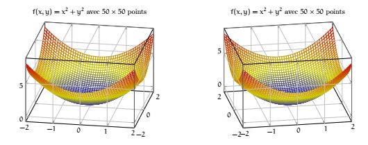
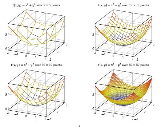
La représentation sous différent angle de vue permet aussi de mieux appréhender la fonction. %Représentation graphique des fonctions à plusieurs variables